How to Run Verlet: An Example |
|---|
| Running Verlet is very simple, but before you run the executable, there are five things you must know. |
|
| 1) The initial temperature in reduced units. The temperature in reduced units defined here is equal to epsilon divided by the Boltzmann constant, where epsilon is the energy constant in the equation for the Lennard-Jones potential. By default, Verlet models a Lennard-Jones fluid, but other potentials can easily be modeled by editing the Force.h file in the Verlet/ directory, and recompiling the sources. Typical values for the initial temperature range from 0.5 to 1.5. |
| 2) The number of particles involved in the simulation. This is a positive integer that is a perfect cube. Examples are 64, 125, 216, and 343. Verlet initially places the particles on a simple cubic lattice, and uses periodic boundary conditions to calculate the distances between the particles. A non-cubic integer will cause the program to produce unpredictable results. |
| 3) The average number density of the fluid that you intend to model. This is a positive floating-point number. The unit of volume is sigma cubed, where sigma is the length constant from the Lennard-Jones potential. If you define another potential, the density will be expressed in terms of that potential's length constant. Typical values are 0.5 to 1.5. |
| 4) The time step for the simulation. This is the time used in the integration of the particle positions in the simulation. Typical values are 1e-5 to 0.01. Due to the Lyapunov instability of a system with such a large number of degrees of freedom, the results will not improve significantly through the use of shorter time steps. Values like 0.001 or 0.001953125=2^-9, will yield good results. | |
| 5) The number of time steps to carry out in the simulation. This is a positive integer. To evaluate the equilibrium properties of the system you are modeling, this number must be much greater than the equilibration time for the system. Using a time step of 0.001, the equilibration time is usually on the order of a few thousand time steps. In some cases 2000 time steps will be sufficient, while in others it will be necessary to run a more than 100,000 time steps which may take more than an hour to complete on a 2004 workstation. The number of time steps must be a power of two if you want to use the FlyvbjergPetersen.exe program to estimate the error on the sample averages. |
|
A Specific Example |
| The graphs below were produced by entering an initial temperature of 0.728, a particle density of 0.8442, 125 for the number of particles, 0.001 for the time step, and running 2^16=65536 time steps. To run the executable, simply type "./Verlet.exe" at the command line in the directory where you have installed Verlet. The program will prompt you to enter values for the quantities described above. I suggest starting with the values given here. Using these values, we are attempting to reproduce the results given in Case Study 4 of Chapter 4 of Understanding Molecular Simulation by Frenkel and Smit. |
|
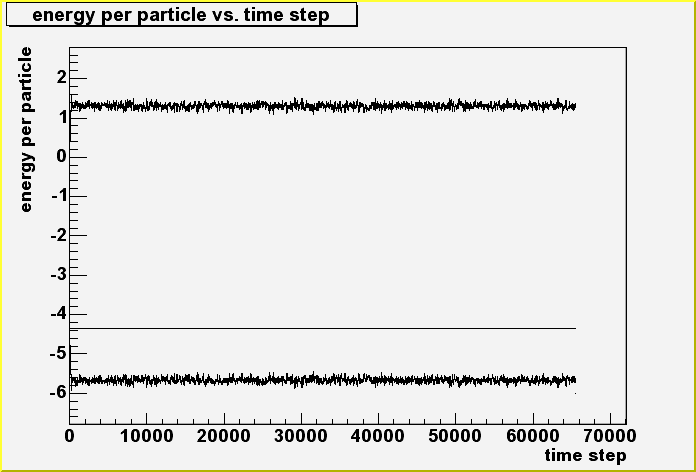
| Running Verlet.exe, yields two output files in the output/ directory. These files are "Energy.dat" and "RadialDistribution.dat". Let us first take a look at Energy.dat. It is a text file with three columns of numbers. The first column lists the kinetic energy per particle at each time step. The second column lists the potential energy per particle at each time step, while the third column lists the total energy per particle at each time step. If you have ROOT installed on your system, you can use the PlotEnergy.C ROOT script to plot these energies. If you do not have ROOT, you'll need to configure whatever plotting program you use to read the Energy.dat file and plot these energies as a function of the time step. The graph of these energies produced by ROOT is below. |
|
 |
|
| There are three curves in the graph above. The top noisy curve that fluctuates around 1.4 is the kinetic energy per particle curve. The flat line at about -4.4 is the total energy per particle curve, and the bottom noisy curve that fluctuates about -5.6 is the potential energy per particle curve. Notice that the the total energy per particle remains constant throughout the simulation. This is a characteristic of a time-reversible algorithm such as the Verlet algorithm, and is required by energy conservation. Although the resolution of the graph is not high enough, if the resolution were high enough, one would see that it takes about 1000 time steps for the system to equilibrate. |
|
| The next graph shows the error on the average potential energy as a function of the the blocking M used in the blocking method described by Flybjerg and Petersen in Reference 1. The data for this graph were generated by the FlybjergPetersen.exe program in the output/ directory and plotted by the PlotError.C ROOT script. |
|
 |
|
| In the graph above sigma is an estimate for the error on the mean value for the potential energy calculated by averaging the potential energy per particle over all time steps after equilibration. In the blocking method of Flyvbjerg and Petersen, one calculates the standard deviation per degree of freedom of a quantity until a plateau is reached where the standard deviation per degree of freedom does not appear to increase significantly by further recursive blocking. The plateau where this occurrs is used as an estimate for the error on the mean value. For example, in the graph above for M=6 to M=9, there is a plateau at about sigma=0.0026. Therefore, we estimate the error on the mean value for the potential energy to be 0.0026. The error bars are the error on the standard deviation per degree of freedom used in the blocking method. |
|
| The final graph below shows the radial distribution function g(r) for the Lennard-Jones fluid modeled in this simulation well after the system has equilibrated. This graph was produced by the PlotRadialDistribution.C ROOT script. Aside from the noise, the graph closely resembles the graph in Figure 4.5 of Understanding Molecular Simulation by Frenkel and Smit. The noise in the graph is due to the fact that only 125 particles were used in the simulation. The radial distribution function is calculated by placing the distances between all pairs of particles calculated using periodic boundary conditions in histogram bins and dividing this number by the number expected in an ideal gas. The graph below comes from a histogram with 256 bins. The noise will fade away as the number of particles is increased. For example, the histogram from which the graph below was generated has 15500 entries, but if we had used 1000 particles in the simulation, the histogram would have had 999000 entries. |
|

|


